If you have been reading up on machine learning and/or deep learning, you have probably encountered Kullback-Leibler divergence [1]. It is commonly used to measure loss in machine learning - and often used in the form of cross-entropy [2]. Now, they are not the same thing, but are close. If these concepts made your eyes glaze over, if you wished there was a more approachable tutorial on these topics, then you are in the right place.
To explain these concepts and build some intuition and python code, let's start with some red and blue balls, and discrete probability distributions.
Lets say you have a bag of full of red and blue balls. Now, lets assume that the bag has 10 red balls and 15 blue balls. So that means it has \frac{10}{10 + 15} or 40% red balls and 60% blue balls. Another way to say this is that if you closed your eyes, and pulled one ball from this bag without looking or cheating, there is a 40% chance, technically probability, that you will pull out a red ball. Similarly, the probability of drawing a blue ball is 60% or 0.6. In probability parlance, the ball we are drawing is a the random variable. Because the ball can take only limited set of colors (2 in this case), we say that it has discrete states. A mathematical function that represents this is the discerete probability distribution of the two states. It shows how colored balls are distributed in between the states.
Here is some code to generate this function:
import numpy as np

np.random.seed(8) # To ensure you get same results on your machine

def redball_blueball(count=1):
'''
Generates a red or a blue ball
By default generates only one ball, but could generate more if desired
'''
bag = np.random.random(count) # generate a bag of balls with count balls
# now lets convert this bag into labels
# we assume that everything that has a value of 0.4 or below is a red ball
# and any value above 0.4 is a blue ball
return ['red' if (x <= 0.4) else 'blue' for x in bag.tolist()]
Lets try it out:
>>> print redball_blueball(10)

['blue', 'blue', 'blue', 'blue', 'red', 'red', 'blue', 'blue', 'blue', 'blue']

>>> print redball_blueball(10)

['blue', 'blue', 'blue', 'blue', 'blue', 'blue', 'red', 'blue', 'red', 'red']

>>> print redball_blueball(10)

['red', 'blue', 'red', 'red', 'red', 'red', 'red', 'blue', 'red', 'blue']
Yes, it was not a copy-paste mistake, I did run it three times. This was to show that even though the expectation from a random number generator is truly random numbers, their distribution may not be in any given window. The bigger the window, the closer it is to the expected distribution. Lets try it out:
from collections import Counter

np.random.seed(8) #reset our random number generator

bag_10 = redball_blueball(10)

bag_100 = redball_blueball(100)

bag_1000 = redball_blueball(1000)

bag_10000 = redball_blueball(10000)

print Counter(bag_10)

print Counter(bag_100)

print Counter(bag_1000)

print Counter(bag_1000)
On my machine, this is what I get:
Counter({'blue': 8, 'red': 2})

Counter({'blue': 65, 'red': 35})

Counter({'blue': 598, 'red': 402})

Counter({'blue': 5937, 'red': 4063})
So, the ratio of red to blue is 20%: 80%, 35%:65%, 40.2%:59.8% and 40.63:59.37%. Larger number of balls drawn make the distribution gravitate to the desired distribution. But it is not exact. Ideally, we want to a ratio of 40%:60%. Before we move forward, lets contrast this with machine learning. Suppose you were trying to classify images into cats and not cats. Then these two possibilities correspond to the red ball and blue ball scenario above. Number of balls corresponds to total number of images that need to be classified. To judge the accuracy of effectiveness of your machine learning algorithm, you need to contrast it's predictions vs that actual number. This corresponds to the numbers our random number code generates above vs the expected answer, which was 40:60. In training the machine learning algorithm, the objective is to minimize this difference. This difference in machine learning literature is referred to as the loss or error. To use this evaluation metric, an objective numerical measure is required that provides a way to measure the difference between these two distributions. This is what KL divergence provides.
Before we delve into the math, lets intuitively figure this out. In the case of red/blue balls, the actual distribution is {0.4, 0.6}. We have other candidate distributions in {.2, 0.8}, {.35, .65}, {.402, .598}, {.4063, .5937}. We want to evaluate each one of them as to how similar they are to the actual distribution. Just by looking at the values, we can say that the third pair is probably the closest, while the first one is the farthest. Now lets try to see if the math of KL divergence, through scipy also supports our intuition. As it is defined, KL divergence measures how far apart these distributions are. So, if the value of divergence is really small, then they are very close. If the number is high, then they are far apart.
>>> from scipy import stats
>>> print stats.entropy(pk=[0.2, 0.8], qk=[0.4, 0.6])
0.0915162218494
>>> print stats.entropy(pk=[0.35, 0.65], qk=[0.4, 0.6])
0.00529177256922
>>> print stats.entropy(pk=[0.402, 0.598], qk=[0.4, 0.6])
8.32873065998e-06
>>> print stats.entropy(pk=[0.4063, 0.5937], qk=[0.4, 0.6])
8.25454404685e-05
As we can see from the results above, our intuition is borne out in the calculation of KL divergence.
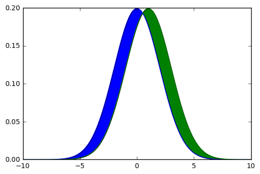
Lets try to understand this more formally. KL Divergence is a measure of how one probability distribution diverges from a second expected probability distribution [3]. To explain in simple terms, consider the code below. We take two distributions and plot them. In the graph, the areas where these two distributions do not overlap are shaded.
import matplotlib.pyplot as plt
x_axis = np.arange(-10, 10, 0.001)
# Mean = 0, SD = 2.
dist_a = stats.norm.pdf(x_axis,0,2)
# Mean = 1, SD = 2
dist_b = stats.norm.pdf(x_axis,1,2)
plt.plot(x_axis, dist_a)
plt.plot(x_axis, dist_b)
plt.fill_between(x_axis, dist_a, dist_b, where=dist_b>=dist_a, facecolor='green', interpolate=True)
plt.fill_between(x_axis, dist_a, dist_b, where=dist_b<=dist_a, facecolor='blue', interpolate=True)
plt.show()
KL Divergence between two distributions
KL Divergence computes the shaded area shown above. Given two probability distributions q(x) and p(x), where the former is the modeled/estimated distributions (for example redball_blueball() function above) and latter the actual of expected distribution, KL Divergence for discrete variables is defined as:
D_{KL}(P||Q) = \Sigma_{i} P(i) log\frac{P(i)}{Q(i)} … (1)
Now we know that log(\frac{x}{y}) = log(x) - log(y). Using this expansion above,
D_{KL}(P||Q) = \Sigma_{i} P(i) log P(i) - \Sigma_{i} P(i)log Q(i) … (2)
We will use this expansion just a little bit later to explain the difference between cross entropy and KL divergence in machine learning. For now, lets code the computation of KL Divergence:
>>> actual = np.array([0.4, 0.6]) # actual number of red and blue balls
>>> model1 = np.array([0.2, 0.8]) # numbers we got above in 10 samples
>>> model2 = np.array([0.35, 0.65]) # numbers we got above for 100 samples
>>>
>>> kl1 = (model1 * np.log(model1/actual)).sum()
>>> print "Model 1: ", kl1
Model 1: 0.0915162218494
>>> kl2 = (model2 * np.log(model2/actual)).sum()
>>> print "Model 2: ", kl2
Model 2: 0.00529177256922
As you can see, our implementation numbers match with those of scipy that we used above. Implementing KL Divergence in python took only one line of code! Well, not really. There many conditions to be considered for a real implementation, but hopefully this gives an idea of how this works.
Before we wrap up, let's pick up the thread on cross-entropy and KL Divergence. Cross-Entropy loss is used commonly in deep learning and machine learning as the loss function for one of many class problems. Ideally, KL divergence should be the right measure, but it turns out that both cross-entropy and KL Divergence both end up optimizing the same thing.
What is cross entropy? Lets take two distributions, whereQ(x) is the estimated distribution, and P(x) is the actual distribution. Cross entropy merely measures where there is disagreement:
H(P, Q) = -\sum_iP(i)log Q(i) ...(3)If you compare this to equation (2) above, there is another term that depends on $$ P(x)$$ only as well. Since $$ P(x)$$ is the actual values, or training data, it can be considered a constant for the problem (technically that term is called the entropy of $$ P(x)$$). Hence, optimizing one optimizes the other. Computationally, it is simpler to compute only the cross-entropy. This particular term is same as log loss in logistic regression. I bet that sounded a lot more familiar.
Hopefully, this gave you good intuition about how KL Divergence works. Go forth and diverge!
References
[1] Kullback, S., and Leibler, R. A. (1951). On information and sufficiency. The Annals of Mathematical Statistics, 22(1), 79-86. Sourced from: https://projecteuclid.org/euclid.aoms/1177729694
[2] From Wikipedia: https://en.wikipedia.org/wiki/Cross_entropy
[3] From Wikipedia: https://en.wikipedia.org/wiki/Kullback%E2%80%93Leibler_divergence


